ANOVA
Analysis of variance (ANOVA) refers to various statistical methods used to compare the means of independent groups of interest in order to assess whether the groups are part of some larger population.
There are various forms of ANOVA, with the simplest form being a one-way ANOVA, which is a type of statistical hypothesis test that uses F-tests and the F-distribution to test the equality of the means of three or more groups. One-way ANOVA can be thought of as an extension of the independent t-test; an independent t-test is used to compare the means of two groups, while one-way ANOVA can be used for 3 or more groups. Other forms of ANOVA include two-way ANOVA, analysis of covariance (ANCOVA), multivariate analysis of variance (MANOVA), and more. This article discusses one-way ANOVA.
One-way ANOVA
One-way ANOVA, also referred to as unidirectional ANOVA, is used under the following conditions:
- The observations are independent: the value of one observation does not affect the value of another.
- The populations are normally distributed.
- The variances of the populations are the same among groups. This is also referred to as the data having homogeneity of variance.
If the above conditions are not met, the results of the test may not be reliable. If the conditions are met, an F-test (along with standard statistical hypothesis testing methods) can be used to compare variances and assess whether a given set of means are all equal. The procedure is generally as follows:
- State the null (H0) and alternative (Ha) hypotheses.
- Select a significance level, α.
- Calculate the F-statistic.
- Determine the critical value for the selected significance level.
- Compare the F-statistic to the critical value to assess whether or not to reject the null hypothesis.
A key part of a statistical hypothesis test is the calculation of the test statistic. In the case of a one-way ANOVA, the test statistic is the F-statistic. The F-statistic is a ratio of variances. Specifically, it is the ratio of the between-group variability, denoted MSbetween, to the within-group variability, MSwithin:

The between-group variability is a measure of how much the means of the groups vary relative to the overall mean, while the within-group variability measures the degree to which the individual datum comprising each group varies relative to the mean of their respective group. MSbetween can be computed using the following formula

where SSbetween is the sum of squares between the mean of each group and the mean of the sampling distribution of means and dFbetween = k - 1 is the degrees of freedom for k groups.
Similarly, MSwithin can be computed as:

where SSwithin is the sum of squares between individual values in the groups and the mean of the respective group and dFwithin = n - k is the degrees of freedom for n observations.
Generally, the closer an F-statistic is to 1, the more evidence there is that the null hypothesis should not be rejected, since a ratio of 1 indicates little difference between the means.
Example
A fitness company wants to compare the efficacy of their various weight loss programs. Participants are grouped into programs A, B, or C. Samples of 5 participants are collected from each group and the mean weight loss (in pounds) from each sample is shown in the table below.
| A | B | C |
|---|---|---|
| 5 | 4 | 10 |
| 6 | 8 | 6 |
| 4 | 2 | 5 |
| 9 | 3 | 9 |
| 15 | 11 | 11 |
 |
 |
 |
The mean of the sampling distribution of means is (7.8 + 5.6 + 8.2)/3 = 7.2 pounds.
Conduct a one-way ANOVA test at a significance level of α = 0.05 to assess whether there is a statistically significant difference between means that would provide evidence for one program being more effective than another.
The null hypothesis and alternative hypotheses are as follows:
| H0: participants lost the same amount of weight in all programs. |
| Ha: participants lost different amounts of weight in all programs. |
To compute the F-statistic, first compute MSbetween and MSwithin.
MSbetween:
 |
 |
 |
 |
 |
 |
MSwithin:
 |
 |
 |
 |
 |
 |
 |
 |
 |
 |
 |
 |
Thus, the F-statistic can be calculated as:

The next step in the hypothesis test is to compare the F-statistic to the critical value, which can be determined by referencing a partial F-distribution table for the chosen significance level (0.05) and the appropriate degrees of freedom (2 for MSbetween and 12 for MSwithin):
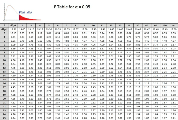
Referencing the table, df1 = 2 and df2 = 12. The value in the 12th row and 2nd column of the table is 3.89. Thus, F(0.05, 2, 12) = 3.89. Comparing this to the calculated F-statistic of 0.72, since 0.72 is less than 3.89, it does not fall in the critical region (indicated in the graph above in red), and there is insufficient evidence to reject the null hypothesis, indicating that the efficacy of the weight loss programs are equivalent.