Riemann sum

A Riemann sum is a method used for approximating an integral using a finite sum. In calculus, the Riemann sum is commonly taught as an introduction to definite integrals. It is used to estimate the area under a curve by partitioning the region into shapes (whose areas are typically simple to compute) similar to the region being measured. The area of these shapes are then added to estimate the area under the curve; most typically, rectangles of even spacing and width are used, though this does not have to be the case.

Since the shapes being used won't exactly match the shape of the region, there will be some error. This error can be reduced by using a larger number of shapes with smaller width; the smaller the width of the rectangles, the more closely they can represent the shape of the region, and the more accurate the estimation of the area. For example, the area under the curve from x = 0 to x = 3 is estimated in each of the graphs below using 4, 10, and 20 rectangles.

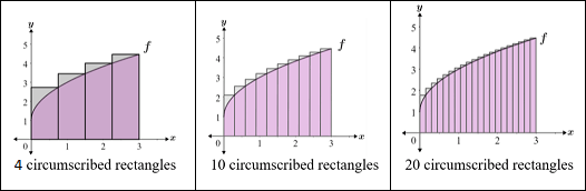
As can be seen from the figure, the higher the number of rectangles used, the more accurate the representation of the area under the curve. This is the basis of the definition of a Riemann sum.

Definition of a Riemann sum

A Riemann sum is defined using summation notation as follows

where represents the width of the rectangles (), and is a value within the interval such that is the height of the rectangle. Thus, represents the area of a given rectangle in the Riemann sum, and the choice of determines which type of Riemann sum (left, right, or midpoint) is being used. for each type of Riemann sum is depicted in the figure below:

Riemann sums and definite integrals

Riemann sums are used to approximate definite integrals; the larger the number of partitions (n), the more accurate the approximation. As the number of partitions approaches infinity, Δx approaches 0. Assuming that it were possible to achieve an infinite number of partitions, the Riemann sum would no longer be an approximation. Rather, the sum would be the exact value of the area under the curve. In other words, the limit of a Riemann sum as Δx approaches 0 over an interval [a, b] is equal to the definite integral over that interval, or:

Note that since Δx approaches 0, it does not matter whether a left, right, or midpoint Riemann sum is used; the limit will still have the same value regardless which point is chosen since they all converge.

Types of Riemann sums

There are a number of different types of Riemann sums. One of the ways in which Riemann sums differ is the choice of , which affects the point at which the curve intersects the partition.

Left Riemann sum

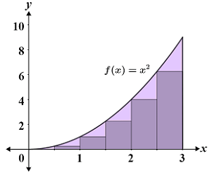
The left Riemann sum involves approximating a function through use of its left endpoint; this means that the left endpoint of the partition is the point that intersects the curve. The figure below depicts a left Riemann sum for f(x) = x² over the interval [0, 3]; the region is partitioned using 6 rectangles of equal width.

The Riemann sum, S, can be expressed as follows:

Since equally spaced rectangles are used in this example, Δx is the same for each partition, and we can use the following expression to determine Δx:

,

where a and b are the endpoints and n is the number of partitions (rectangles in this case). Note that this expression can be used to determine the width of the partition for any case in which all the partitions have equal width. Thus,

,

and the sum can be evaluated as follows:

Thus, the area under the curve is approximately 6.875 units. Referencing the figure, this is an underestimation of the area since all of the partitions are under the curve. Generally, a left Riemann sum will result in an overestimation if f(x) is only decreasing on the given interval, such as it would be left of the y-axis of f(x) = x². If f(x) is only increasing on the interval, such as it is in this example, the left Riemann sum results in an underestimation.

Right Riemann sum

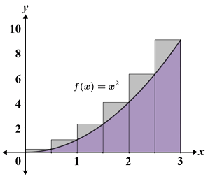
The right Riemann sum is similar to the left Riemann sum with the key difference being that the function is approximated using the right endpoint; this means that the right endpoint of the partition is the point that intersects the curve. The figure below depicts a right Riemann sum for f(x) = x² over the interval [0, 3]; the region is partitioned using 6 rectangles of equal width.

Since the rectangles all have equal width,

,

and the right Riemann sum can be computed as:

Thus, the area under the curve is approximately 11.375 units. Referencing the figure, this is an overestimation because the partitions extend above the curve. Generally, the right Riemann sum results in an underestimation if f(x) is only decreasing on the given interval. When f(x) is only increasing on the interval, as in this example, the right Riemann sum results in an overestimation of the area.

Midpoint rule

Unlike the left and right endpoints, which are relatively simple to read off the graph, it is necessary to calculate the midpoint by summing the left and right endpoints, then dividing by 2. When using the midpoint rule,

.

The figure below depicts a Riemann sum using the midpoint rule for f(x) = x² over the interval [0, 3]; the region is partitioned into 6 rectangles of equal width.

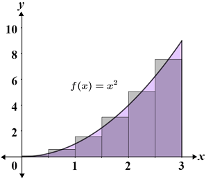
When using the midpoint rule, the function intersects the partition at the midpoint of the partition. For this example, for each of the 6 partitions is as follows:

Since all of the rectangles have equal width,

,

and the Riemann sum can be computed as follows:

Thus, the area under the curve is approximately 8.938 units. This is an underestimation of the actual area under the curve, though it is difficult to discern this from only examining the figure. Generally, the midpoint rule underestimates the area under the curve if the function is always increasing over the interval, and overestimates the area if the function is always decreasing over the interval.