Calculus
Calculus is a branch of mathematics that is the study of change. We use calculus to help explain the physical world around us. Disciplines such as physics, statistics, economics, and medicine, use calculus to not only explain the problems and issues that confront them, but also to construct models that can be used to predict future events or to describe past events.
The two main branches of calculus are differential calculus and integral calculus. At its base, differential calculus deals with rates of change and considers the slope of a function at a point, while integral calculus considers the area under and between the curves of a function.
In practice, calculus involves the thorough study of limits, as an understanding of limits is necessary in order to tackle topics such as continuity, derivatives, integrals, series, and more.
Limits
A limit is the value that a function approaches as its input value approaches some value. It provides information about a function's behavior near a point, rather than at that point. For example, the limit of the function  as x approaches 2 is denoted as follows:

Notice that in this particular example, it is not possible to evaluate the function at x = 2, since x = 2 results in the denominator of the function being 0, and the function being undefined. However, while we cannot determine the value of the function at x = 2, we can use limits to determine the value that the function approaches as it gets closer and closer to 2.
Limits can be determined in a number of ways, such as graphically, algebraically, or numerically. The table below depicts a numerical approach.
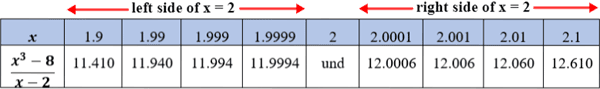
The table shows values of f(x) as x approaches 2 from the left and right side. Based on the table, as x approaches 2 from either side, f(x) approaches a value of 12. Thus:

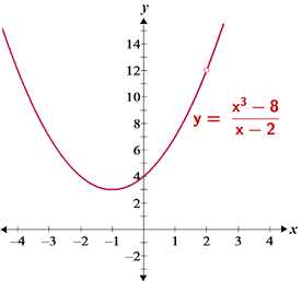
A graph of f(x) shows the same result. Note again that f(x) is undefined at x = 2, as depicted by the open circle on the curve:
It is also possible to simplify f(x) to determine the limit algebraically:
 |
 |
 |
|
 |
Plugging x = 2 into the simplified expression,

which is the same result obtained using the graphical and numerical methods. It is worth noting that it is also possible for a limit to not exist. Generally, a limit exists if the function approaches the same value from either side. Below are some conditions under which a limit does not exist:
- The one-sided limits (the limit as x approaches some value from one side, e.g. from -∞) are not equal.
- The value the function approaches is not finite, e.g. infinity.
- The function oscillates, so the function does not approach any particular value, e.g. the sine function.
If a limit exists, the above methods, as well as others, may be used to compute the limit. The choice of method when determining a limit is dependent on a number of factors including the function and the resources available.
Continuity
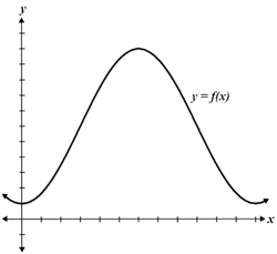
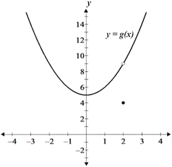
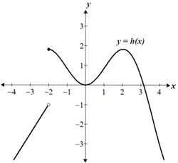
Informally, a function is said to be continuous if its graph is a single unbroken curve; in other words, it has no discontinuities such as asymptotes, jump discontinuities, or removable discontinuities. Given the graph of a function, it is usually relatively straightforward to determine whether the graph is continuous or discontinuous. The figure below shows 3 graphs, only one of which is continuous:
|
|
|
| Continuous | Removable discontinuity | Jump discontinuity |
As can be seen, the first graph is continuous because there are no breaks in the graph; it is a parabola with no discontinuities. On the other hand, the second and third graphs are discontinuous for different reasons. The second graph has what is referred to as a removable discontinuity. A removable discontinuity is one in which the one-sided limits from the negative and positive directions exist, are equal, and are finite at a given point, but the value of the function at said point is not equal to the limit. The third graph has a jump discontinuity in which the one-sided limits from the negative and positive directions are not equal.
Formally, a function f(x) is continuous at some point x = a if:
- f(a) is defined


Thus, a function is continuous if the above is true for all values within its domain.
Continuity gives way to many important concepts in calculus, including the intermediate value theorem. The intermediate value theorem states that for a continuous function f over an interval [a, b], if c is a value between a and b (a ≤ b ≤ c), there must exist at least one value f(c) such that f(c) is between f(a) and f(b):
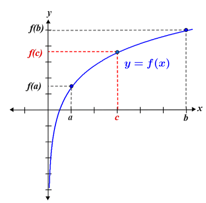
As can be seen from the graph, c is a value between a and b, and f(c) is between f(a) and f(b). The intermediate value theorem states that this is true for any value between a and b for a continuous function.
Derivatives
In general terms, the derivative of a function is a measure of how rapidly a function's output changes relative to a change in the input value. The study of, and calculation of derivatives is a large part of early calculus. Derivatives are important because they have many real world applications in areas such as engineering, economics, health care, and more. As a basic example, a function may model an object's position with respect to time; the derivative of that function at a specific point in time would provide the object's rate of change in position at that point in time (its velocity). Although this is only one general example, this use of the derivative alone can be applied to many real world problems.
Mathematically, the derivative is the slope of the line tangent to a curve at a given point, which can be determined using limits and the formula for the slope of a line. The figure below shows the graph of a function, f(x).
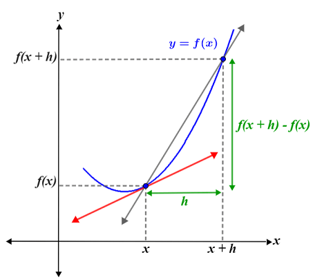
Two points on the curve, (x, f(x)) and (x + h, f(x + h)), as well as the secant line between those points are also shown. The slope, m, of the secant line can be determined as:

The red line shown is the line tangent to the curve at x. Its slope can be determined by using the equation for the slope of the secant line, then decreasing h until it is infinitesimal (very small, e.g. close to 0), such that Δx between x and x + h is so small that it is essentially 0. In other words, we find the limit of the slope of the secant line as h approaches 0, which gives us the slope at a single point. The grey lines in the figure below show the progression of secant lines formed as h approaches 0:
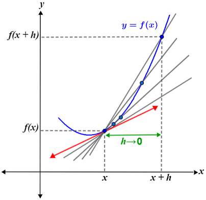
This is the basis of the definition of a derivative, denoted f'(x):

The derivative is also denoted in a number of different ways such as:

The limit definition of a derivative is often cumbersome to use. For this reason, the derivatives of many commonly used functions have been generalized, though the table below is not exhaustive:
| Power rule |
|---|

|
| Trigonometric rules |

|

|

|

|

|

|
| Logarithm/exponent rules |

|

|

|

|
| Product/quotient rules |

|

|
Integrals
The integral of a function represents the area between the curve of the function and the x-axis. The concept of an integral is useful because many real world problems can be modeled using functions, so the area under the curve of a function can represent many practical things such as volumes, areas, and more.
An integral is sometimes referred to as an antiderivative because the operation of integration is the opposite of differentiation. Thus, integrals and derivatives are closely related.
Integrals are often discussed as indefinite or definite integrals. A definite integral has upper and lower limits over which a function is integrated and results in a value that is the area under the curve between the upper and lower limit. An indefinite integral has no such limits, and the result of an indefinite integral is the antiderivative of the given function.
The integral of a function f(x) is denoted as follows:

Similarly, a definite integral over the interval [a, b] would be denoted as:

The indefinite integrals for many commonly used functions are shown in the table below:
| Power rule |
|---|

|
| Trigonometric rules |

|

|

|

|

|

|

|

|

|

|
| Logarithm/exponent rules |

|

|

|