Intermediate value theorem

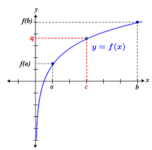
Let f(x) be a continuous function at all points over a closed interval [a, b]; the intermediate value theorem states that given some value q that lies between f(a) and f(b), there must be some point c within the interval such that f(c) = q. In other words, f(x) must take on all values between f(a) and f(b), as shown in the graph below.

It is worth noting that the intermediate value theorem only guarantees that the function takes on the value q at a minimum of 1 point; it does not tell us where the point c is, nor does it tell us how many times the function takes on the value of q (it can occur only once, or many times). Consider the example of the change in temperature (which is a continuous function) in a fictional city over the course of a 24-hour period, as depicted in the figure below:

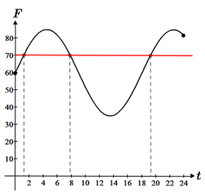
The temperature recorded at 12 am and 11:59 pm are 60°F and 80°F respectively. We can see from the graph that the temperature fluctuates wildly over the 24-hour interval; the temperature even goes above and below our known values at the endpoints of the interval. All the intermediate value theorem tells us is that given some temperature that lies between 60°F and 80°F, such as 70°F, at some unspecified point within the 24-hour period, the temperature must have been 70°F. This makes sense because we intuitively know that even if the temperature were to change rapidly, the temperature cannot change from 60°F to 80°F without having been 70°F at some point.

The intermediate value theorem is important mainly for its relationship to continuity, and is used in calculus within this context, as well as being a component of the proofs of two other theorems: the extreme value theorem and the mean value theorem. It can also be used to examine various properties of a function, such as whether or not a function has a 0.

Example

f(x) = x² - x - 7 is continuous for all real numbers. f(3) = -1 and f(4) = 5. Using the intermediate value theorem, determine whether or not f(x) has a 0 over the interval [3, 4].

The function fits the criteria for use of the intermediate value theorem since it is continuous over the interval in question. Thus, the function takes on all values between -1 and 5. Since 0 is between -1 and 5, we know that f(x) does have a 0 at some point c within the closed interval.

There are a number of ways to find the 0, but using the intermediate value theorem alone, we cannot determine the position of the zero. For the sake of completeness, we find the zero(s) of the function using the quadratic formula:

-0.19 is outside the closed interval, so even though it is a zero of the function, we are not interested in this particular zero. 3.19 is within the interval [3, 4], so we confirm that f(x) has a zero at c = 3.19. The figure below is a graph of f(x) over the interval [3, 4] that shows the position of the zero: