Continuous
A function is continuous if its graph has no breaks or holes. One way to test this informally is to trace/draw graph of the function; if it is possible to trace the function over a given interval without having to lift the pencil, the function is continuous over that interval; otherwise, the function is not continuous over that interval. Below are a few examples of continuous and discontinuous functions:
|
|
|
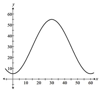
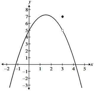
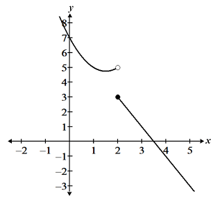
| a. Continuous | b. Removable discontinuity | c. Jump discontinuity |
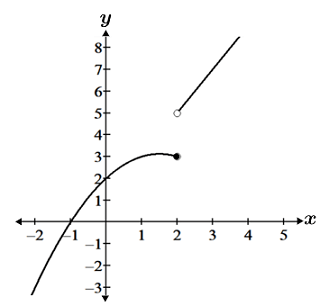
The function shown in panel a is continuous over its entire domain. The other two functions shown are both discontinuous at a point. In panel b, the function has a removable discontinuity (a hole) at x = 3, while the function in panel c has a jump discontinuity at x = c. The functions are otherwise continuous at all points except those specifically mentioned. As can be seen, when discussing continuity, it is necessary to state the interval over which the function is continuous, since a function may be continuous over large intervals and only discontinuous at a single point.
Formal definition
To define continuity formally, we must make use of limits. For a function to be continuous at a point x = a, it must meet the following criteria:
- f(a) must be defined.
 .
. .
.
Note that the above tests the continuity of a single point. For a function to be continuous over its entire domain, the above must be true for every point within the domain of the function.
Example
Determine whether  is continuous at x = 3.
1. Determine whether f(a) is defined:

Thus, f(a) is not defined at x = 3, and therefore not continuous at x = 3, even though we can confirm that its limit exists at that point.
2. For completeness, we can determine that the limit exists:
 |
 |
 |
|
 |
|
 |
3. Since f(a) = undefined, and  :
:
 ,
,
and we can again confirm that f(x) is not continuous at x = a.
Types of discontinuities
Discontinuities are categorized as removable or non-removable discontinuities.
- Removable discontinuity - the limit still exists, even though the function has a discontinuity.
- Non-removable discontinuity - the function has a discontinuity such that the limit does not exist.
Removable discontinuities
Removable discontinuities are so named because it is possible to re-define the function such that the function becomes continuous, thus "removing" the discontinuity. The figure below shows a graph with a removable discontinuity at x = 2.
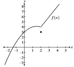
In the above function, there is a discontinuity at the point (2, 4), but the function is defined at x = 2, and the limit also exists at x = 2. This is an example of a removable discontinuity because we can re-define the function at the point x = 2 such that f(2) = 4, while retaining the definition of the rest of the function for all other x values. This re-definition makes the function continuous at x = 2.
Non-removable discontinuities
Non-removable discontinuities can take on multiple forms, such as jump discontinuities and infinite discontinuities. Non-removable discontinuities are so named because the limit does not exist, so unlike removable discontinuities, it is not possible to re-define the function in a way that will make it continuous. The figure below shows a jump discontinuity and an infinite discontinuity:
|
|
| a. Jump discontinuity | b. Infinite discontinuity |
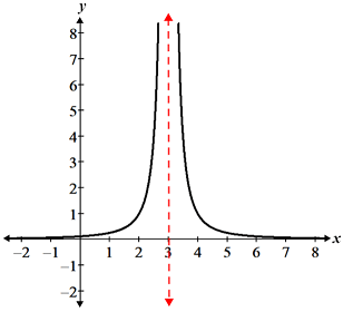
The function shown in panel a exhibits a jump discontinuity. Even though it is defined at x = 2 and we can determine the left-hand and right-hand limits, since the left and right-hand limits are not equal, the limit does not exist. The function in panel b exhibits an infinite discontinuity at x = 3 due to the vertical asymptote. The limit does not exist at this point because the function approaches infinity from both the left and right-hand sides.
Intermediate value theorem
The concept of continuity is used throughout the study of calculus. One important consequence of continuity is the intermediate value theorem. The intermediate value theorem states that for a continuous function f(x) over the interval [a, b], if q is a value between f(a) and f(b), the function will take on the value q at least once at some point c within the interval [a, b]. Refer to the figure below:
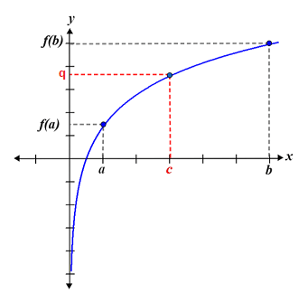
In the figure, q is a value that lies between f(a) and f(b). We can see that the function is continuous over the interval [a, b]. Although we cannot determine the point at which the function will take on the value q, because the function is continuous, we know that it will take on the value q at least once at some point c.
It is important to note that the intermediate value theorem cannot be used to determine the value of c. We can only conclude that some point c exists such that the function takes on the value of q at c. Also, the intermediate value theorem only guarantees that there is at least one point c. It is possible for a function to take on the value of q at multiple points over the interval, but it is not possible to use the intermediate value theorem to determine the number of times the function takes on the value q.
It is also worth noting that the intermediate value theorem only tells us that f(x) will take on the value of q if q lies between f(a) and f(b). If q does not lie between f(a) and f(b), the intermediate value theorem cannot be used to draw any conclusions about whether or not f(x) takes on the value of q. In other words, even if some value q does not lie between f(a) and f(b), f(x) may take on the value of q within the interval multiple times, or not at all.
Example
Consider the function f(x) = sin(x) over the interval [0, 5]. Use the intermediate value theorem to determine whether or not f(x) takes on the values ±0.707 within the given interval.
f(0) = 0, and f(5) = -0.959. Since 0.707 does not lie between 0 and -0.959, we cannot use the intermediate value theorem to determine whether or not f(x) takes on the value of 0.707. However, -0.707 does lie between 0 and -0.959, and since 0 > -0.707 > -0.959, we can conclude using the intermediate value theorem that f(x) does indeed take on the value of -0.707 at some point within the interval [0, 5]. Refer to the graph below:
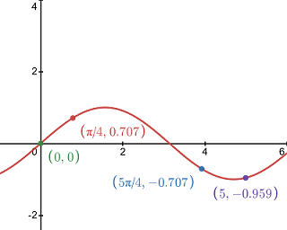
Referencing the graph, we can see that f(x) takes on the value of -0.707 at x = 5π/4. Looking at the graph however, we can see that f(x) does actually take on the value of 0.707 at π/4. This demonstrates the fact that the intermediate value theorem can only be used to verify that the function will take on a given value given the appropriate conditions. It would have been incorrect to draw the conclusion that f(x) doesn't take on the value of 0.707 based on the fact that 0.707 didn't lie between f(0) and f(5).