Chi square test
A chi-square test is a type of statistical hypothesis test that is used for populations that exhibit a chi-square distribution.
There are a number of different types of chi-square tests, the most commonly used of which is the Pearson's chi-square test. The Pearson's chi-square test is typically used for data that is categorical (types of data that may be divided into groups, e.g. age, race, sex, age), and may be used to test three types of comparison: independence, goodness of fit, and homogeneity. Most commonly, it is used to test for independence and goodness of fit. These are the two types of chi-square test discussed on this page. The procedure for conducting both tests follows the same general procedure, but certain aspects differ, such as the calculation of the test statistic and degrees of freedom, the conditions under which each test is used, the form of their null and alternative hypotheses, and the conditions for rejection of the null hypothesis. The general procedure for a chi-square test is as follows:
- State the null and alternative hypotheses.
- Select the significance level, α.
- Calculate the test statistic (the chi-square statistic, χ2, for the observed value).
- Determine the critical region for the selected level of significance and the appropriate degrees of freedom.
- Compare the test statistic to the critical value, and reject or fail to reject the null hypothesis based on the result.
Chi-square goodness of fit test
The chi-square goodness of fit test is used to test how well a sample of data fits some theoretical distribution. In other words, it can be used to help determine how well a model actually reflects the data based on how close observed values are to what we would expect of values for a normally distributed model.
To conduct a chi-square goodness of fit test, it is necessary to first state the null and alternative hypotheses, which take the following form for this type of test:
| H0: The data follow a given distribution. |
| Ha: The data do not follow a given distribution. |
Like other hypothesis tests, the significance level of the test is selected by the researcher. The chi-square statistic is then calculated using a sample taken from the relevant population. The sample is grouped into categories such that each category contains a certain number of observed values, referred to as the frequency for the category. As a rule of thumb, the expected frequency for a category should be at least 5 for the chi-square approximation to valid; it is not valid for small samples. The formula for the chi-square statistic, χ2, is shown below

where Oi is the observed frequency for category i, Ei is the observed frequency for category i, and n is the number of categories.
Once the test statistic has been calculated, the critical value for the selected level of significance can be determined using a chi-square table given that the degrees of freedom is n - 1. The value of the test statistic is then compared to the critical value, and if it is greater than the critical value, the null hypothesis is rejected in favor of the alternative hypothesis; if the value of the test statistic is less than the critical value, we fail to reject the null hypothesis.
Example
Jennifer wants to know if a six-sided die she just purchased is fair (each side has an equal probability of occurring). She rolls the die 60 times and records the following outcomes:
| Number rolled | Frequency |
|---|---|
| 1 | 13 |
| 2 | 7 |
| 3 | 14 |
| 4 | 6 |
| 5 | 15 |
| 6 | 5 |
Use a chi-square goodness of fit test with a significance level of α = 0.05 to test the fairness of the die.
The null and alternative hypotheses can be stated as follows:
| H0: the die is fair. |
| Ha: the die is not fair. |
Since there is a 1/6 probability of any one of the numbers occurring on any given roll, and Jennifer rolled the die 60 times, she can expect to roll each face 10 times. Given the expected frequency, χ2 can then be calculated as follows:
| # | Observed frequency |
Expected frequency |
Oi-Ei | (Oi-Ei)2 | (Oi-Ei)2/Ei |
|---|---|---|---|---|---|
| 1 | 13 | 10 | 3 | 9 | 0.9 |
| 2 | 7 | 10 | -3 | 9 | 0.9 |
| 3 | 14 | 10 | 4 | 16 | 1.6 |
| 4 | 6 | 10 | -4 | 16 | 1.6 |
| 5 | 15 | 10 | 5 | 25 | 2.5 |
| 6 | 5 | 10 | -5 | 25 | 2.5 |
| Sum | 60 | 60 | N/A | N/A | 10.0 |
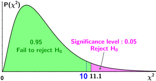
Thus, χ2 = 10. The degrees of freedom can be found as n - 1, or 6 - 1 = 5. Thus df = 5. Referencing an upper-tail chi-square table for a significance level of 0.05 and df = 5, the critical value, is 11.07. Since the test statistic is less than the critical value, we fail to reject the null hypothesis. Thus, there is insufficient evidence to suggest that the die is unfair at a significance level of 0.05. This is depicted in the figure below.
Chi-square test of independence
The chi-square test of independence is used to help determine whether the differences between the observed and expected values of certain variables of interest indicate a statistically significant association between the variables, or if the differences can be simply attributed to chance; in other words, it is used to determine whether the value of one categorical variable depends on that of the other variable(s). In this type of hypothesis test, the null and alternative hypotheses take the following form:
| H0: there is no statistically significant association between the two variables. |
| Ha: there is a statistically significant association between the two variables. |
Though the chi-square statistic is defined similarly for both the test of independence and goodness of fit, the expected value for the test of independence is calculated differently, since it involves two variables rather than one. Let X and Y be the two variables being tested such that X has i categories and Y has j categories. The number of combinations of the categories for X and Y forms a contingency table that has i rows and j columns. Since we are assuming that the null hypothesis is true, and X and Y are independent variables, the expected value can be computed as

where ni is the total of the observed frequencies in the ith row, nj is the total of the observed frequencies in the jth column, and n is the sample size. χ2 is then defined as

where Oij is the observed value in row i and column j, Eij is the expected value in row i and column j, p is the number of rows, and q is the number of columns in the contingency table. Also, note that p represents the number of categories for one of the variables while q represents the number of categories for the other variable.
For a chi-square test of independence, the degrees of freedom can be determined as:
df = (p - 1)(q - 1)
Once df is known, the critical value and critical region can be determined for the selected significance level, and we can either reject or fail to reject the null hypothesis based on the results. Specifically:
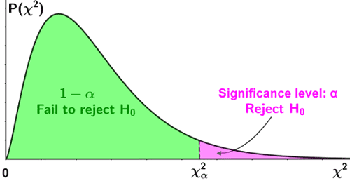
- For an upper-tailed one-sided test, use a table of upper-tail critical values. If the test statistic is greater than the value in the column of the table corresponding to (1 - α), reject the null hypothesis.
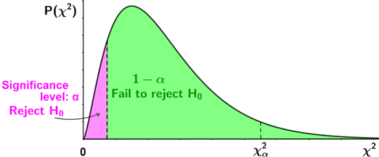
- For a lower-tailed one-sided test, use a table of lower-tail critical values. If the test statistic is less than the value in the column of the table corresponding to α, reject the null hypothesis.
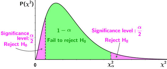
- For a two-sided test, use a table for upper-tail critical values for the upper tail, and a table for the lower-tail critical values for the lower tail.
- Upper tail: if the test statistic is greater than the value in the column corresponding to (1 - α/2), reject the null hypothesis.
- Lower tail: if the test statistic is less than the value in the column corresponding to α/2, reject the null hypothesis.
The figure below depicts the above criteria for rejection of the null hypothesis.
| One-tailed tests | |
|---|---|
| Upper-tailed test |
|
| Lower-tailed test |
|
| Two-tailed test | |
|
|
Example
A survey of 500 people is conducted to determine whether there is a relationship between a person's sex and their favorite color. A choice of three colors (blue, red, green) was provided, and the results of the survey are shown in the contingency table below:
| Color | ||||
|---|---|---|---|---|
| Sex | Green | Blue | Red | Row sum |
| Male | 100 | 85 | 68 | 253 |
| Female | 77 | 65 | 105 | 247 |
| Column sum | 177 | 150 | 173 | 500 |
Conduct a chi-square test of independence to test whether there is a relationship between sex and color preference at a significance level of α = 0.05.
The null and alternative hypotheses can be stated as follows:
| H0: a person's favorite color is independent of their sex. |
| Ha: a person's favorite color is not independent of their sex. |
Eij is computed for each row and column as follows:


Thus:
| Color | ||||
|---|---|---|---|---|
| Sex | Green | Blue | Red | |
| Male | O11 = 100 E11 = 89.56 |
O12 = 85 E12 = 75.9 |
O13 = 68 E13 = 87.54 |
|
| Female | O21 = 77 E21 = 87.44 |
O22 = 65 E22 = 74.1 |
O23 = 105 E23 = 85.46 |
|
The chi-square statistic is then computed as:
 |
 |
 |
|
 |
|
 |
The degrees of freedom is computed as:
df = (2 - 1)(3 - 1) = 2
Thus, using a chi-square table, the critical value for α = 0.05 and df = 2 is 5.99. Since the test statistic, χ2 = 13.5, is greater than the critical value, it lies in the critical region, so we reject the null hypothesis in favor of the alternative hypothesis at a significance level of 0.05.