Z-score
A Z-score (also referred to as a standard score) indicates the number of standard deviations that an observed value is from the mean in a standard normal distribution. For example, a Z-score of 1 indicates that the observed value is 1 standard deviation from the mean. A value can be above, below, or equal to the mean, indicated by the sign of the Z-score:
- A positive Z-score indicates that the value is above (right of) the mean.
- A negative Z-score indicates that the value is below (left of) the mean.
- A Z-score of 0 indicates that the value is equal to the mean.
How to calculate a Z-score
There are a few different formulas for calculating a Z-score. Given that the population mean and standard deviation are known, a Z-score can be calculated using the following formula

where μ is the mean, σ is the standard deviation, and x is the observed value.
In cases where the population mean and standard deviation are not known, they can be estimated by a sample mean and standard deviation. The formula for calculating the Z-score remains the same, with the exception that the population parameters are replaced with their corresponding sample statistics:

where x is the sample mean, s is the sample standard deviation, and x is the observed value.
Another form of the Z-score formula is used when calculating the Z-score for a sampling distribution of means, rather than for a single value; in such cases, the standard error must be taken into account. The Z-score for a sampling distribution of means can be calculated using the formula

where x is the sample mean, μ is the population mean, σ is the population standard deviation, and n is the sample size.
Example
A student in a class of 210 students scores a 65 on an exam in which the class average was a 53 with a standard deviation of 6. Given that the test scores are normally distributed, calculate the Z-score of the student's score on the exam.
Since the population mean and standard deviation are known, the Z-score can be calculated as follows:

The student's score on the exam corresponds to a Z-score of 2. Since the Z-score is positive, this means that the student's score is 2 standard deviations above the mean. If we had only looked at the student's raw score of 65, we may have concluded that the student did not perform well on the exam. However, the Z-score indicates that the student actually performed well on the exam relative to their peers, since their score is 2 standard deviations above the mean. It is for this reason that many exams are graded on a curve, taking the distribution of scores into account. The figure below shows the normalized distribution of test scores, as well as the position of the student's Z-score within the distribution:
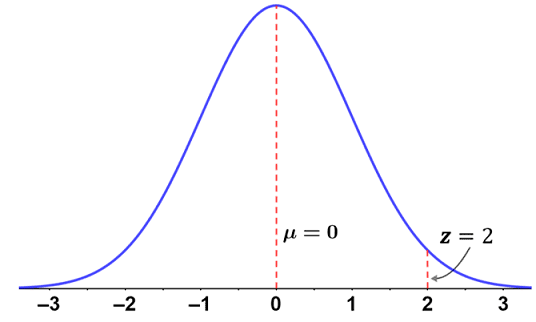
As is characteristic of normally distributed data, the further an observed value lies from the mean, the less likely it is to occur. Based on the graph, we can again confirm that the student's score of 65 was significantly better than the rest of their class. Using Z tables, it is possible to determine the percentile in which a score lies.
Applications of Z-scores
The above example shows that we can discern information about observed data based on the position of a Z-score in a standard normal distribution. Z-scores can also be used in conjunction with Z tables to determine the percentage of scores above or below a given Z-score and the probability of an outcome lying in a given interval. Z-scores are also used as part of Z-tests to test whether an observed outcome is statistically significant.
Z-test
A Z-test is a type of statistical hypothesis test that is used when the test statistic exhibits a normal distribution and the standard deviation of the population is known. It is used to determine whether there is a significant difference between an observed mean and the mean under the null hypothesis, H0. The process involves stating a null hypothesis and an alternative hypothesis, selecting a significance level, and calculating a Z-score for the observed value. Once the Z-score is calculated, it can be used to draw conclusions about the statistical significance of an experiment using either the p-value method or the critical value method:
- p-value: the Z-score is used in conjunction with Z-tables to calculate a p-value, which indicates the probability of obtaining test results that are at least as extreme as the observed results under the assumption that the null hypothesis is true. In order to use a p-value to draw conclusions about a test-statistic, it is compared to the significance level, α (typically 0.01, 0.05, or 0.10). If the p-value is less than α, the null hypothesis is rejected in favor of the alternative hypothesis.
- Critical value: the critical value(s) for the given significance level can be determined using a Z-table. Critical values are the boundaries of the critical region(s). If the Z-score of the observed value lies within a critical region, the null hypothesis is rejected in favor of the alternative hypothesis.
Z tables
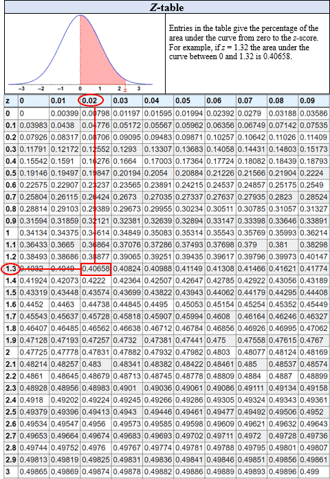
Z tables are tables that provide the probability that an observed statistic lies above, below, or between values on a standard normal distribution (or Z distribution). They are useful because any normal distribution can be converted to a standard normal distribution, and since the central limit theorem states that many test statistics have normal distributions given that the sample is large enough, Z tables are widely applicable. For this reason, a variety of Z tables have been constructed so that the probabilities of various test statistics can be easily determined without having to integrate the probability density function of a normal distribution each time. The figure below shows a cumulative from mean Z table:
Example
Referencing the example above,
- use a Z table to determine the percentage of students who scored above and below a 65 on the exam.
- what is the probability of a student who took the exam later scoring between a 55 and 65, given the same exam and conditions?
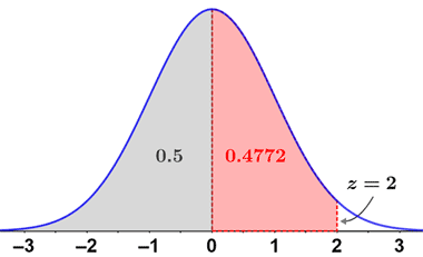
i. In the above example, we determined that a score of 65 corresponds to a Z-score of 2. Referencing the cumulative from mean Z table, a Z-score of 2 corresponds to a probability of 0.47725. This is the probability of a score lying between the mean and a Z-score of 2. However, the probability of scores below the mean must also be added. Since 50% of scores lie below the mean, and 50% of scores lie above the mean, the probability of a score lying below a Z-score of 2 is
P(Z < 2) = 0.50 + 0.47725 = 0.97725
and the probability of a score lying above is:
P(Z > 2) = 1 - P(Z < 2) = 1 - 0.97725 = 0.02275
Thus, there is approximately a 97.7% chance of scoring below a 65, and a 2.3% chance of scoring above a 65. The figure below shows the area under the standard normal distribution represented by P(Z < 2):
ii. The probability of scoring between a 55 and 65 is given by the area under the standard normal distribution between their respective Z scores. First, convert both scores to Z-scores:


Referencing the Z table, a Z-score of 0.33 corresponds to a probability of 0.1293. A Z-score of 2 corresponds to a probability of 0.47725. The area between the two can be found as their difference:
0.47725 - 0.1293 = 0.34795
Thus, there is approximately a 35% chance of the student scoring between a 55 and 65 on the exam.