Null hypothesis
The null hypothesis (H0) is the basis of statistical hypothesis testing. It is the default hypothesis (assumed to be true) that states that there is no statistically significant difference between some population parameter (such as the mean), and a hypothesized value. It is typically based on previous analysis or knowledge.
The null hypothesis is used for various purposes, such as to verify statistical assumptions, to verify that multiple experiments are producing consistent results, to directly advance theories, and more.
Most commonly, the null hypothesis is used to state the equality between two or more variables, such as a drug and a placebo. This equality is then tested in a statistical hypothesis test. Generally, the null hypothesis is the hypothesis that the researcher is attempting to disprove, though this is not necessarily always the goal. It is contrasted with the alternative hypothesis (Ha), which is a statement that there is some difference (value is greater than, less than, or not the same), and seeks to provide evidence that any observed differences are statistically significant, rather than due to random variation.
For example, the null hypothesis may state that the GPA of students at a given high school is not better than the state average. The corresponding alternative hypothesis may state that the GPA of students at a given high school is better than the state average, and a hypothesis test would then be conducted to determine whether there is sufficient evidence to reject the null hypothesis in favor of the alternative hypothesis.
Notation
Mathematically, the null hypothesis is denoted as H0, and is stated as
H0: μ = μ0
where μ0 is the assumed or hypothesized population mean, and μ is the mean of the population from which samples are drawn. Since the null hypothesis is a statement that there is no difference between these population parameters,
μ - μ0 = 0
The alternative hypothesis generally takes one of three forms:
| Ha: μ > μ0 |
| Ha: μ < μ0 |
| Ha: μ ≠ μ0 |
H0 can also be stated as an inequality:
H0: μ > μ0
The corresponding alternative hypothesis is stated as:
Ha: μ ≤ μ0
Statistical hypothesis testing
A statistical hypothesis test adheres to the following general procedure:
- State the null and alternative hypotheses.
- Select a significance level, α (the probability of rejecting the null hypothesis when the null hypothesis is true), and the appropriate test statistic.
- Conduct the appropriate test and determine the critical region of the corresponding distribution.
- z-test
- t-test
- chi-squared test
- F-test
- Calculate the observed value of the test statistic.
- Reject the null hypothesis in favor of the alternative hypothesis if the observed value lies within the critical region. Otherwise, do not reject the null hypothesis.
Alternatively, instead of using critical regions, it is possible to calculate the p-value and compare it to the chosen significance level:
- If the p-value is less than or equal to the significance level, reject the null hypothesis in favor of the alternative hypothesis.
- If the p-value is greater than the significance level, do not reject the null hypothesis.
Note that the aim of this type of hypothesis test is to determine whether there is evidence to reject the null hypothesis in favor of the alternative hypothesis at a given significance level. This is not the same as proving or accepting an alternative hypothesis, since there may be evidence for the alternative hypothesis at one significance level, but not another. Also, if there is insufficient evidence for the alternative hypothesis, we fail to reject the null hypothesis, rather than accepting it; it is not possible to accept the null hypothesis.
Example
The national average SAT score, calculated for all juniors, was 1150 with a standard deviation of 75. A sample of 35 juniors from a given high school had an average score of 1250. Assuming a significance level of 0.05, use a Z-test to determine whether the difference between the average score of the class of 35 and the national average is statistically significant.
1. State the null and alternative hypotheses:
H0: μ = 1150
Ha: μ ≠ 1150
2. The selected significance level is 0.05, and test scores follow a normal distribution, so it is appropriate to calculate the Z-score of the test statistic and conduct a Z-test.
3. Since we want to determine if any difference exists, a two-tailed test is appropriate, which means that the 0.05 critical region is broken up into two critical regions comprising an area of 0.025 each; the critical regions for a two-tailed Z-test given a 0.05 significance level are:
Z < -1.96 and Z > 1.96
4. Calculate the Z-score of the observed value:

5. Since the Z-score of the observed value does not lie within the critical region (as shown in the figure below), we fail to reject the null hypothesis.
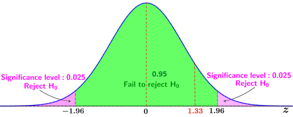
Failing to reject the null hypothesis suggests that there is not a statistically significant difference between the average scores of the class of 35 and the national average at a significance level of 0.05.
A significance level α of 0.05 means that there is a 5% chance of rejecting the null hypothesis when the null hypothesis is true. When this occurs, the error is referred to as a type I error, or a false positive. In cases where the opposite occurs, and we fail to reject the null hypothesis when it is false, it is referred to as a type II error, as summarized in the table below:
| H0 is true | H0 is false | |
|---|---|---|
| Reject H0 | Type I error | Correct inference |
| Fail to reject H0 | Correct inference | Type II error |