Confidence interval
A confidence interval is a range of values that describes the uncertainty inherent in forming an estimate of a population parameter based on a random sample of said population. It is a range of likely values of a given population parameter based on a selected confidence level. For example, a confidence level of 95% indicates that, given that the same procedure and constraints are used to generate the confidence interval, 95% of the computed confidence intervals will contain the population parameter. Thus, the confidence interval does not reflect the variability of the population parameter. Rather, it provides a range of values that are likely to include the population parameter based on the random error of the sample.
Confidence level
A confidence level provides the proportion of confidence intervals that contain the true population parameter. A confidence level is selected prior to examining the data. The most commonly used confidence level is 95%, though 90% and 99% are also used.
Based on the central limit theorem, the sampling distribution of sample means for a given population is normally distributed for large samples (typically n>30). Furthermore, the empirical rule states that for a normally distributed random variable, 95% of the values lie within 2 standard deviations of the mean. Thus, given a normally distributed random variable with sample mean, x, a confidence interval of x ± 2σx will contain the population mean, μ, if x falls within two standard deviations of the true population mean. This is depicted in the figure below.
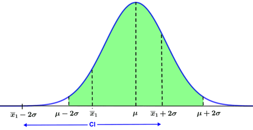
The confidence interval computed using the sample mean, x1, and a confidence level of 95% is shown in the figure. This confidence level means that any confidence interval computed using the same constraints will contain the population mean, μ, 95% of the time. Only values of the sample mean that lie outside of the area shaded in green will fail to include the true population parameter, and this will occur 5% of the time.
Generally, a higher confidence level results in a wider, but less precise confidence interval. The example above applies to a confidence level of 95%. The computation of a confidence interval is dependent on the confidence level, which determines the margin of error.
Computing a confidence interval
A confidence interval is computed by adding and subtracting the margin of error (MOE) to the test statistic. For a sample mean, x, the confidence interval (CI) can be expressed as
CI = x ± MOE
where the computation of the margin of error is dependent on whether the population standard deviation is known. If it is not known, it can be estimated using the sample standard deviation. For a normally distributed random variable with known standard deviation, the margin of error is computed using the formula

where z* is the critical value of the Z distribution for the given confidence level, σ is the standard deviation, and n is the sample size. If the standard deviation is estimated using a sample standard deviation, a Student's t distribution is used instead of a Z distribution, and the margin of error is computed using the formula

where t* is the critical value of the Student's t distribution, s is the sample standard deviation, and n is the sample size.
Example
A survey of of 100 U.S. adults finds that they watch an average of 15 hours of TV per week. Given that the population standard deviation is known to be 2 hours, compute a confidence interval for the average number of hours of TV watched at a 95% confidence level.
Since the sample size is larger than 30, we can assume that the data is normally distributed and compute z* since the population standard deviation (σ = 2) is known. The critical value, z*, is dependent on the selected confidence level and whether a one-sided or two-sided confidence level is appropriate. Since we are concerned with deviations on either side of the mean, rather than on only one side, a two-sided confidence interval is appropriate in this case. z* can be determined using a Z table by finding the Z-score of the value on either side of the Z distribution that corresponds to a probability of α/2, where α, the significance level, is computed by subtracting the confidence level from 1:
α = 1 - 0.95 = 0.05
Thus, z* is the Z-score on either side of the Z distribution corresponding to a probability of 0.025, or:
z* = 1.96
Refer to the Z table page for more information on using Z tables. The margin of error can then be computed as

and the confidence interval given a sample mean of 15 is:

Based on this confidence interval, we may infer that U.S. adults watch an average of between 14.61 and 15.39 hours of TV per week.
Confidence intervals are also commonly depicted graphically. For example, the figure below depicts the confidence interval 6 ± 3:
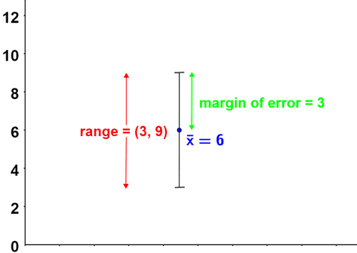
The sample mean is represented by a dot on the graph, and the margin of error is represented by line segments extending above and below the sample mean. Note that graphs of confidence intervals may also take on a horizontal form, rather than a vertical one.
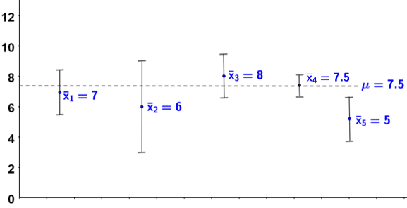
Typically, the confidence intervals of multiple random samples are graphed, each of which may or may not include the population mean, which is represented by a dotted line; the multiple random samples are dispersed across this line. In the figure below, the population mean is μ = 7.5, and 5 confidence intervals are shown, 4 of which include the population mean.
Common misunderstandings
There are a number of common misunderstandings surrounding confidence intervals, typically concerning the probability represented by the confidence level. Since confidence intervals are so widely used and discussed in statistics, it can be helpful to be aware of these misunderstandings.
- Confidence intervals are commonly used to make statements of probability such as "Given a 95% confidence level, there is a 95% chance that the population parameter lies within the confidence interval." This statement is false. A confidence interval, once computed, either contains or does not contain the population parameter. A confidence level of 95% indicates that repeated samples collected using the same procedure will result in confidence intervals that contain the population parameter ~95% of the time. The 95% confidence level is a statement about the reliability of the procedure used to compute the confidence interval, and is not related to the probability of the population parameter being within a specific confidence interval.
- A confidence level is sometimes mistaken for representing the percentage of sample data that lies within the confidence interval. This is not the case. A confidence interval of 95% does not indicate that 95% of the sample data lies within the confidence interval.
- A confidence interval is sometimes mistaken as providing the range of all possible values that the sample statistic can take on. This is not the case, as the range is based on the sample mean and the standard error, which will vary between samples.
- A calculated 95% confidence interval does not represent an interval within which the sample parameter from a repeat of the experiment lies. For example, given the confidence interval 6 ± 3 calculated using a 95% confidence level, this interval cannot be used to make a statement such as "Given that the same procedure is used, there is a 95% probability that the sample parameter of a subsequent experiment will lie within the interval 6 ± 3." Again, a 95% confidence level indicates that given that the same procedure is repeated, the computed confidence intervals will tend to contain the population parameter 95% of the time. A 95% confidence interval is simply a confidence interval that was computed for a 95% confidence level.