Central limit theorem
The central limit theorem states that in many situations, as the sample size of an experiment gets larger, the sampling distribution will tend towards a normal distribution. This is true regardless of the actual distribution of the population variable, which means that probabilistic and statistical methods that are used with normal distributions can still be applied in certain cases that involve other types of distributions.
The central limit theorem makes it possible to make inferences about independent random variables in a population by repeatedly sampling the population. This is because the mean of the sampling distribution (also referred to as the mean of the means) of a given population variable will approximate the mean of the actual population given a sufficiently large sample size.
For example, consider a loaded die that is rolled 10,000 times. The frequency of the outcomes is shown in the histogram below.
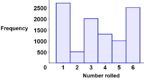
The frequency distribution is clearly not that of a typical fair 6-sided die (which would have more evenly distributed outcomes). The average number rolled based on the frequency distribution is:

This is the average of the entire population. Given that a random sample of 30 rolls is taken from the population, the sample mean, x1 might equal 3.3; subsequent samples will result in different sample means, xi, that may equal 3.1, 2.7, 4.1, 3.5, etc. If we were to continue taking many (thousands) random samples of 30 rolls from the population, the central limit theorem states that the distribution of the sample means might look like the histogram below,
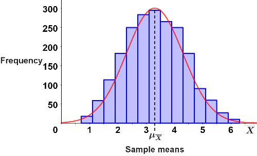
which takes the form of a normal distribution, shown by the bell shaped curve in red. As can be seen, the mean of the sample means, μx, lies around the center of the distribution; approximately as many sample means lie to the left or right of μx, which also has a value close to that of the population mean, μ. The central limit theorem can be similarly used to approximate other population statistics.
Given that the variance of the population is known, it is possible to find the sample variance, σx2:

where σ2 is the variance of the population and n is the sample size used in the sampling distribution. Based on the equation, we can see that as the sample size increases, the sample variance decreases, since the population variance is a fixed value.
Summary of the central limit theorem
Some of the key takeaways regarding the central limit theorem are shown below:
- The sampling distribution of the mean follows a normal distribution for a relatively large sample size. Note: use a sample size of n ≥ 30 for a population that is not normally distributed, or n ≤ 30 when the population is normally distributed.
- The mean of the sampling distribution of the means is approximately the same as the population mean.
- The variance of the sampling distribution of the means is less than that of the population when n > 1.
- The larger the sample size, the smaller the variance of the sampling distribution of the mean.
The example below demonstrates how the central limit theorem can be used to estimate a population statistic.
Example
Suppose that the average amount of stimulus money that a worker in the U.S. received each month during the 2020 pandemic was $1200 with a standard deviation of $400. If 100 workers are sampled, what is the probability that they received more than an average of $1250 each month in stimulus money?
Since the sample size is 100, the central limit theorem applies, and we can reasonably theorize that the sampling distribution of the mean is normally distributed, allowing us to find the mean and standard deviation of the sample as follows:
The mean of the sampling distribution of the mean, μx, is equal to the population mean, μ, or 1200. Thus, the sample variance and standard deviation can be computed as:


Knowing the standard deviation and mean is useful because it enables us to determine certain statistics, such as a z-score, which can give us an idea of how far a given data point is from the mean. Because the conditions for using the central limit theorem have been met, we can use a z-score and our collected sample to determine the probability that the sample of 100 workers received more than $1250 each month. Let X be a sample mean. The probability that X is greater than $1250 can be calculated by finding the z-score and using a z-table:

Thus:

Using a z-table, we can determine that:

Thus, the probability that the sample of 100 workers received more than $1250 is approximately 11%.