Sampling distribution
A sampling distribution is the probability distribution of a statistic. It is obtained by taking a large number of random samples (of equal sample size) from a population, then computing the value of the statistic of interest for each sample. Thus, a sampling distribution depicts the range of possible outcomes of a given statistic, as well as their probabilities, for the sampled population.
For example, twenty bags of hard candy are randomly selected from a warehouse to be used for estimating the average number of pieces of candy per bag. This process is repeated 99 more times to produce a sampling distribution of 100 sample means, as shown in the histogram below.
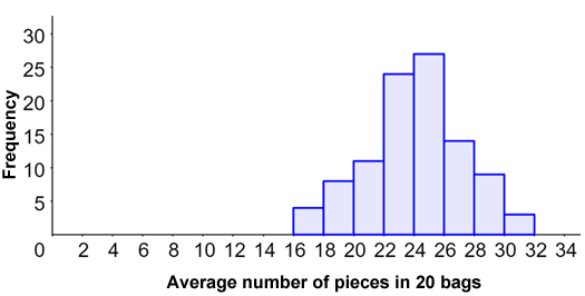
The sampling distribution tells us the number of samples that had a given mean, and can be used to find the probabilities of a given mean occurring. For example, in 5 of the 100 samples, the 20 randomly selected bags had an average of 17 pieces of candy per bag. Thus, there is a 5% (5/100) chance that a bag will contain 17 pieces of candy.
Sampling distributions are important because they allow us to make inferences about a statistical population based on the probability distribution of the statistic, which significantly simplifies what would otherwise be a more complicated statistical process.
Sampling distributions and the central limit theorem
The central limit theorem states that as the sample size for a sampling distribution of sample means increases, the sampling distribution tends towards a normal distribution, regardless of whether or not the population from which the samples are taken has a normal distribution. Thus, the mean of the sampling distribution of the mean is equal to the mean of the population for an arbitrarily large sample size; in other words, μx = μ. The following histogram shows an example of what a sampling distribution of sample means from a large number of random samples might look like:
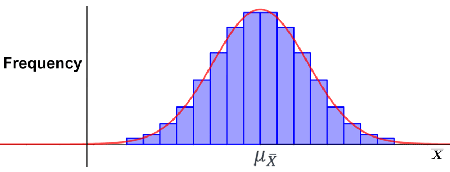
As shown by the curve in red, the histogram tends towards a normal distribution, and the sample means are dispersed approximately equally on either side of the mean, indicating that the mean of the sample means is the same as the mean of the population.
Sampling distributions and the central limit theorem can also be used to determine the variance of the sampling distribution of the means, σx2, given that the variance of the population, σ2 is known, using the following equation:

where n is the size of the samples in the sampling distribution. As can be seen from the equation, as the sample size increases, the sample variance decreases, since the population variance has a fixed value. This is useful because sampling distributions and the central limit theorem allow us to estimate population statistics using sampling distributions.
Example
A population has a mean of 20 and a standard deviation of 8. 50 samples are taken from the population; each has a sample size of 35.
- Find the mean and standard deviation of the sampling distribution of the means.
- Find the probability that the mean of the sample means is between 18 and 22.
i. Since the sample size is relatively large, μx = μ = 20, and the sample sample standard deviation σ can be calculated using the sample variance:


ii. Since the sample size is relatively large, we can also consider the distribution to be normal, so we can use z-scores to determine P(18 < X < 22):

Using a z-table:

Thus, the probability that the mean of the 50 randomly chosen sample means is between 18 and 22 is 86%.