Normal distribution
A normal distribution is a type of continuous probability distribution. It is one of the most commonly used probability distributions, in part because many random variables with unknown distributions can be modeled using a normal distribution. This is largely due to the central limit theorem, which states that the sampling distribution of the sample means of a given population tends towards a normal distribution as the sample size gets larger, regardless of the actual shape of the population's distribution. Thus, many statistical tests can be performed, and inferences can be made about many different populations based on the central limit theorem.
Examples of normally distributed random variables include height, weight, test scores, and more. The graph below shows an example of normally distributed ACT scores for a given year.
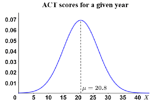
A normal distribution is symmetric about its mean. In the figure above, we can see that the mean, μ, is at the center of the graph, and that 50% of the values lie above the mean, while 50% of the values lie below the mean. Also, the further the scores are away from the mean, the less likely it is for the scores to occur. These are just a few characteristics of a normal distribution; below are others:
- A normal distribution is continuous.
- A normal distribution is symmetric about its mean.
- The mean, median, and mode are equal for a normal distribution.
- The variance of normally distributed data is equally distributed about the mean.
- The graph forms a bell-shaped curve such that the maximum value is the mean.
- The probability of occurrence is lower the further away (left or right) a value is from the mean.
- The area beneath the normal distribution curve is 1, since the probabilities of every outcome must sum to 1.
The general form of the probability density function (pdf) of a normal distribution is

where μ is the mean and σ is the standard deviation of the random variable. The simplest form of the normal distribution is referred to as the standard normal distribution, or Z distribution.
Standard normal distribution
The standard normal distribution is a normal distribution in which the mean (μ) is 0 and the standard deviation (σ) and variance (σ2) are both 1. This simplifies the above probability density function to:

Any normal distribution can be converted to a standard normal distribution, which is useful because a normal distribution can have any range of means or standard deviations, making it difficult to compare various distributions to each other. Consider the two normal distributions shown in the figure below:
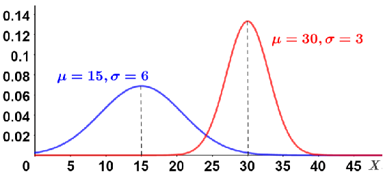
Notice that the shape of the normal distribution varies significantly based on the mean and standard deviation; the smaller the standard deviation, the narrower the curve; the larger the standard deviation, the wider the curve. Standardizing normal distributions, particularly when we want to compare them, removes these differences and allows for a direct comparison, rather than having to consider the different means and standard deviations of the various normal distributions.
Furthermore, standardizing normal distributions allows us to determine the probability that the observations lie above or below a given value using what is referred to as a Z table, rather than having to integrate the probability density function of a normal distribution. Using a Z table is something that can be done conveniently, and relatively simply by hand, rather than requiring the use of computers or calculators.
How to compute a Z score
Any value from a normal distribution can be standardized by converting it to what is referred to as a Z score. A Z score describes an individual value's relationship to the mean of the group of values in terms of standard deviations from the mean. The score itself tells us how many standard deviations a value is from the mean. For example, a Z score of 1 means that the value is 1 standard deviation from the mean.
Z scores can be positive, negative, or 0:
- A positive Z score indicates that a value is above (right of) the mean.
- A negative Z score indicates that a value is below (left of) the mean.
- A Z score of 0 indicates that a value is equal to the mean.
The following formula can be used to convert a value from a normal distribution to a Z score

where μ is the mean, σ is the standard deviation, and x is the value to be converted.
A Z score can also be converted to a percentile, which indicates the score below which a given percentage of the scores in a distribution fall.
Example
John scored a 1310 on the SAT and wants to determine how well he did relative to other students who took the test. The average score was an 1100 with a standard deviation of 250, and the scores are normally distributed. In what percentile did John rank?
First, find the Z score:

The Z score indicates that John's score was 0.84 standard deviations above the mean. Using a Z-table, as shown in the figure below, we can find the probability of a student receiving a score between that of the mean and John's score:
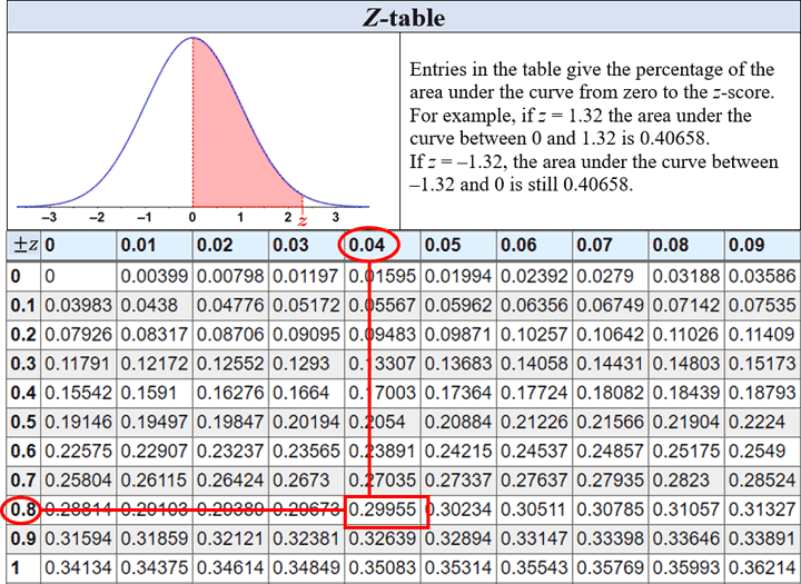
There is a 30% chance of a student receiving a score between the mean and John's score. Since 50% of scores lie below the mean, this percentage is added to determine the total percentage of students who scored below John; this is depicted in the figure below:
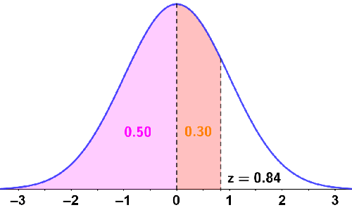
Thus, John's score is in the 80th percentile of test scores, meaning that 20% of students received a score higher than John's.
The empirical rule
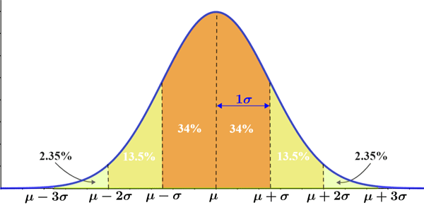
The empirical rule (also referred to as the 68-95-99.7 rule) states that for data that follows a normal distribution, almost all observed data will fall within 3 standard deviations of the mean. More specifically, where μ is the mean and σ is the standard deviation:
- Approximately 68% of observed data falls within 1 standard deviation (Z = ±1) of the mean.
- Approximately 95% of observed data falls within 2 standard deviations (Z = ±2) of the mean.
- Approximately 99.7% of observed data falls within 3 standard deviations (Z = ±3) of the mean.
The empirical rule is represented in the figure below:
The empirical rule is useful for providing a rough estimate of the outcome of an experiment as long as the data follows a normal distribution. It can also be used to determine if a given set of data follows a normal distribution. For example, if it takes an average of 20 minutes in line to be admitted to the venue of a concert, the admission time has a standard deviation of 3.5 minutes, and the data follows a normal distribution, the empirical rule can be used to forecast that given a sample of the people who attended the concert:
- 68% of the admission times would fall within the range of 16.5-23.5 minutes.
- 95% of the admission times would fall within the range of 13-27 minutes.
- 99.7% of the admission times would fall within the range of 9.5 - 30.5 minutes.