Uniform distribution
A uniform distribution is a type of symmetric probability distribution in which all the outcomes have an equal likelihood of occurrence. There are two types of uniform distributions: discrete and continuous. The following table summarizes the definitions and equations discussed below, where a discrete uniform distribution is described by a probability mass function, and a continuous uniform distribution is described by a probability density function.
| Discrete | Continuous |
|---|---|
 |
 |
 |
 |
 |
 |
Discrete uniform distribution
A discrete uniform distribution is one that has a finite (or countably finite) number of random variables that have an equally likely chance of occurring. Examples of experiments that result in discrete uniform distributions are the rolling of a die or the selection of a card from a standard deck. For a fair, six-sided die, there is an equal probability (1/6) of rolling a 1, 2, 3, 4, 5, or 6. Similarly, a standard deck of cards has 52 different cards, so the probability of selecting any one card is 1/52. Also, in both cases, there are distinct outcomes (dice roll or cards), indicating the discrete nature of the events.
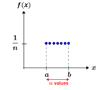
More specifically, let x be a discrete random variable having n values over the interval [a, b]; x has a discrete uniform distribution if its probability mass function (pmf) is defined by:

The graph of a discrete random distribution showing the 7 different outcomes is depicted in the figure below. Each outcome has the same probability (1/n) of occurring, thus the distribution is both uniform and discrete.
Expected value and variance
The expected value and variance are two statistics that are frequently computed. To find the variance, first determine the expected value for a discrete uniform distribution using the following equation:

The variance can then be computed as

where  , and f(x) is the probability mass function (pmf) of a discrete uniform distribution, or
  . Thus:
 |
 |
 |
|
 |
The variance can then be found by plugging E(X2) and [E(X)]^2 into the above equation:
 |
 |
 |
|
 |
|
 |
Example
10 ping pong balls are numbered 1-10 and placed in a bag. One ping pong ball is removed from the bag randomly.
i. Find the expected value and the variance.
ii. Find the probability that the number on the drawn ping pong ball is between 7 and 10.
i. Using n = 10 and the above equation:


ii. The pmf is f(x) = 1/10, and the probability of selecting a ping pong ball numbered between 7-10 is:
 |
 |
 |
Thus, the probability of selecting a ball numbered between 7 and 10 is 20%.
Continuous uniform distribution
A continuous uniform distribution is a type of symmetric probability distribution that describes an experiment in which the outcomes of the random variable have equally likely probabilities of occurring within an interval [a, b]. The probability density function (pdf) of a continuous uniform distribution is defined as follows.
An example of a continuous uniform distribution is shown in the figure below.
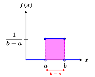
A continuous uniform distribution is also referred to as a rectangular distribution due to the rectangular area formed between a and b. Because a pdf represents the probabilities of all possible outcomes, the area of the shaded area in the graph of the pdf is equal to 1.
Example
It takes a shuttle 20 minutes to travel from stop A to stop B. The shuttle travels between stops A and B continuously throughout the day. What is the probability that a person at stop A will wait more than 8 minutes for the shuttle to arrive?
Let X be a continuous random variable that represents the wait time for a shuttle. Its pdf is:

The probability that X > 8 is represented by the area of the shaded region in the figure below.
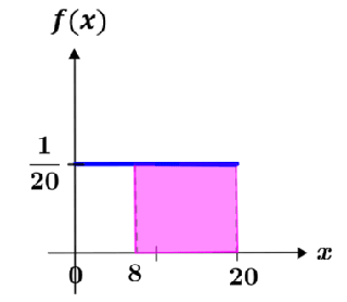
The area of the shaded region can be calculated as:

The area of the shaded region could also have been calculated by integrating over the interval:
 |
 |
 |
Thus, the probability that a person will wait more than 8 minutes is 60%.
Expected value and variance
The expected value of a pdf is given by:

For the pdf of a continuous uniform distribution, the expected value is:
 |
 |
 |
|
 |
|
 |
|
 |
The above integral represents the arithmetic mean between a and b. This is because the pdf is uniform from a to b, meaning that for a continuous uniform distribution, it is not necessary to compute the integral to find the expected value. Instead it is possible to compute the expected value over an interval by finding the arithmetic mean between the two endpoints, which is typically a simpler calculation.
The variance of a random variable can be found using the equation

where

Substituting the pdf for a continuous uniform distribution results in the following:
|
 |
 |
|
 |
|
 |
|
 |
The above can then be substituted into the variance equation to find the variance:
|
 |
 |
|
 |
|
 |
|
 |