Gaussian distribution
A Gaussian distribution, also referred to as a normal distribution, is a type of continuous probability distribution that is symmetrical about its mean; most observations cluster around the mean, and the further away an observation is from the mean, the lower its probability of occurring. Like other probability distributions, the Gaussian distribution describes how the outcomes of a random variable are distributed.
The Gaussian distribution, so named because it was first discovered by Carl Friedrich Gauss, is widely used in probability and statistics. This is largely because of the central limit theorem, which states that an event that is the sum of random but otherwise identical events tends toward a normal distribution, regardless of the distribution of the random variable. Many natural phenomena, such as height, weight, test scores, and others, fit this criteria, and therefore exhibit a normal distribution.
Gaussian function
The graph of a Gaussian function forms the characteristic bell shape of the Gaussian/normal distribution, and has the general form

where a, b, and c are real constants, and c ≠ 0. In a Gaussian distribution, the parameters a, b, and c are based on the mean (μ) and standard deviation (σ). Thus, the probability density function (pdf) of a Gaussian distribution is a Gaussian function that takes the form:

Although the graphs of all Gaussian distributions share the same general bell shape, the parameters of the function affect the overall shape of the graph:
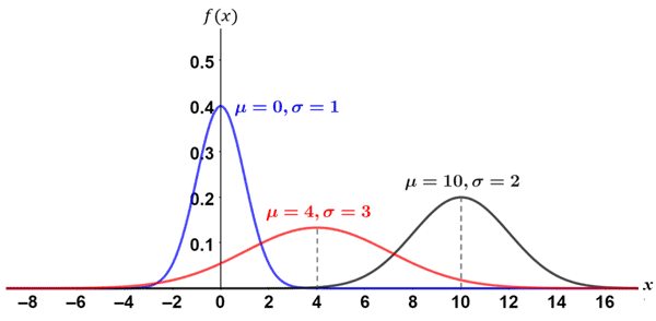
As can be seen from the figure, different μ and σ significantly affect the shape of the graph, making it taller, narrower, or wider, etc. Generally, the larger the standard deviation, the flatter the curve will be because the probability of a given outcome is less likely the further away from the curve an outcome is from the mean. Because different normal distributions can have such different shapes, standardization is often useful. The graph above, shown in blue, is referred to as the standard normal distribution.
Standard normal distribution
A standard normal distribution is the standardized form of a Gaussian distribution in which μ = 0 and σ = 1. It is worth noting that any Gaussian distribution can be converted to a standard normal distribution. This is important because, typically, to determine the probabilities of various outcomes in a probability distribution, it is necessary to integrate the probability density function (pdf) to determine the area under the curve; this is not the case for a standard normal distribution. The figure below shows the graph of a Gaussian distribution.
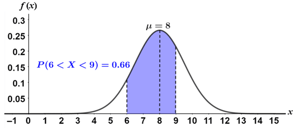
The shaded area represents the area under the curve, or the probability that an outcome will fall between 6 and 9. Integrating the pdf of a Gaussian distribution over this interval yields said probability, but since the pdf of a normal distribution is relatively complicated, it is more common to use calculators or computers to calculate these integrals.
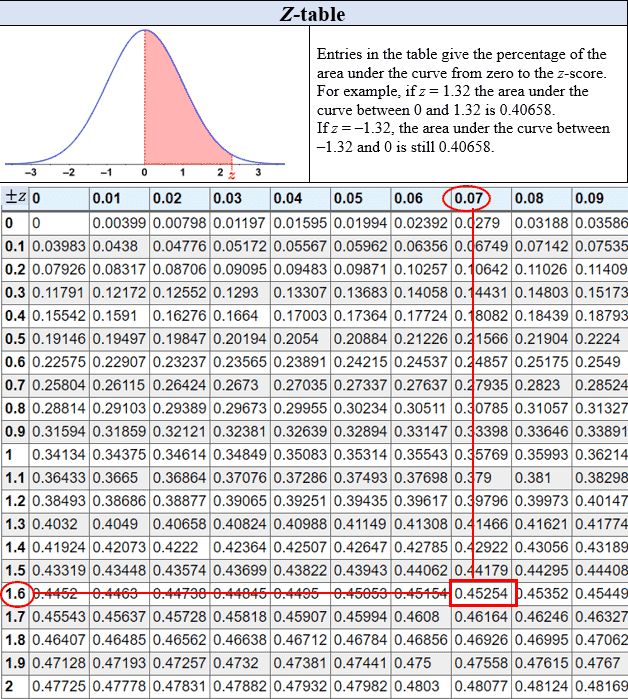
In the case of the standard normal distribution, the probabilities of various outcomes have already been compiled into tables. Thus, rather than having to integrate to determine probabilities of interest, we can simply read the probabilities off of what is referred to as a Z table. This in turn allows us to easily compare different normal distributions.
Converting to a standard normal distribution
Given a random variable X that exhibits a Gaussian distribution, individual values can be standardized using the following formula:

where z is the Z-score, μ is the mean, σ is the standard deviation, and x is the value to be converted. All values in a Gaussian distribution can be converted to Z-scores using this formula, and the resulting distribution is referred to as the standard normal distribution, or Z distribution.
A Z-score indicates the number of standard deviations that a given value is from the mean. For example, a Z-score of 1 indicates that the value is 1 standard deviation from the mean. A Z-score can be positive, negative, or zero.
- A positive Z score indicates that a value is above (right of) the mean.
- A negative Z score indicates that a value is below (left of) the mean.
- A Z score of 0 indicates that a value is equal to the mean.
Z-scores are used in conjunction with Z tables to determine various probabilities.
Example
The average height of 5th graders in a given school district is 52 inches with a standard deviation of 2.4 inches. Assuming that the heights of the 5th graders in the district are normally distributed, find the probability that a 5th grader chosen at random is taller than 56 inches.
First, convert the value of interest to a Z-score:

There are a few different types of Z tables. The Z table in the figure below is a cumulative from mean Z table, meaning that a value in the table represents the probability that an outcome will lie in the interval between the mean (0) and the chosen Z-score (1.67 in this case). Refer to the table below.
Thus, there is approximately a 45% chance that an outcome will lie between a Z-score of 0 and 1.67. However, this is not the probability that a student is taller than 56 inches; to determine this probability, we need to find P(X > 1.67), which we can determine by subtracting the probability we found from 50%. This is because 50% of outcomes lie on either side of the mean (for a normal distribution), so we know that 50% of values lie above the mean, and subtracting the probability we found above from 50% will give us P(X > 1.67). This is depicted in the figure below.
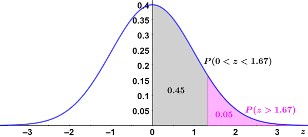
Thus:
0.50 - 0.45 = 0.05 = 5%
Therefore, there is a 5% chance that a student chosen at random will be taller than 56 inches.