Probability distribution
A probability distribution is a function that describes the probabilities of occurrence of the various possible outcomes of a random variable. As a simple example, consider the experiment of tossing a fair coin three times. The possible outcomes of each individual toss are heads or tails. Let the random variable X be the number of tails that result from three flips of a fair coin; the sample space of this experiment is:
{HHH, HHT, HTH, HTT, THH, THT, TTH, TTT}
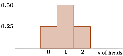
Thus, there is 1 way for 0 tails to occur, 3 ways for 1 tails to occur, 3 ways for 2 tails to occur, and 1 way for 3 tails to occur; the probability distribution is shown in the table below:
| Number of tails | Probability |
|---|---|
| 0 | 1/8 |
| 1 | 3/8 |
| 2 | 3/8 |
| 3 | 1/8 |
The above is an example of a discrete probability distribution. Note that the sum of probabilities must be 1.
All probability distributions can be classified as either discrete probability distributions or continuous probability distributions.
Discrete probability distribution
A probability distribution is either discrete or continuous depending on whether the random variable is discrete or continuous. A discrete variable can only take on distinct values, such as a coin toss landing on either heads or tails, or the number of students in a class. The coin can only land on heads or tails, while the number of students in a class is a specific number, such as 20. There cannot be 20.5 students, 30.7 students, etc.
A discrete probability distribution can be described by a probability mass function (pmf), which provides the probability of occurrence of each value of a discrete random variable. A pmf has the following properties:
- The probability, P, of x ∈ X is: P(X = x) = f(x)
- f(x) ≥ 0 for all x
- The sum of the probabilities of all possible values must equal 1:

There are a number of types of probability mass functions. The pmf used to model the experiment is dependent on the type of experiment. Three examples of commonly used discrete probability distributions include the discrete uniform distribution, binomial distribution, and Poisson distribution.
Discrete uniform distribution
A discrete uniform distribution can be used to represent a random variable that has a finite number of values that have an equally likely chance of occurrence. Rolling a fair 6-sided die is one such example, since each of the 6 faces of the die has an equal probability of occurring on a given toss.
Let X be a discrete random variable with n values over the interval [a, b]. X has a discrete uniform distribution if its pmf is defined by

for x = 1, 2, 3, ... n. It has the following form:
Binomial distribution
A binomial distribution is used to model an experiment in which there are only two possible outcomes. Tossing a fair 2-sided coin is one such example, since the only possible outcomes are heads or tails. Below is an example of a binomial distribution for the experiment of flipping 2 fair coins:
The pmf for a binomial distribution is:

| p is the probability of success of an individual trial |
| q = 1 - p is the probability of failure |
| n is the number of trials |
| x is the number of successes from n trials |
 |
Example
Given that only 20% of all adults can pass a specific cognitive test, what is the probability that of 5 randomly selected adults, 3 of them pass the test?
Since there are only two possible outcomes, pass or fail, we can use the pmf for a binomial distribution to determine the probability, where p = 0.2, q = 0.8, n = 5, and x = 3:
 |
 |
 |
Thus, there is a 5% probability that 3 of the 5 randomly chosen adults will pass the cognitive test.
Poisson distribution
A Poisson distribution can be used to model the probability that an independent event will occur a certain number of times over a specific period of time (or distance, area, volume, etc.). For example, the number of times per month that a particular red light gets run by a car may exhibit a Poisson distribution.
The pmf for a Poisson distribution is

where λ is the mean number of events for the specified period, and e ≈ 2.718 is Euler's number.
Continuous probability distribution
A continuous variable is one that can take on any value within some interval, and a continuous probability distribution is the probability distribution of a continuous random variable. Examples of continuous variables include height and weight. There are upper and lower limits to human height and weight, but within those limits, there are an infinite number of possible heights and weights. For example, two people who measure 5 feet 8 inches tall are unlikely to be exactly the same height. Instead, their height probably varies by some decimal value that cannot be measured precisely.
The probability that a continuous random variable takes on any individual outcome is 0, so unlike discrete probability distributions, continuous probability distributions cannot be represented using a table. Instead, continuous probability distributions are typically represented by a probability density function, which can be used to determine the probability that the random variable will lie within a certain range of values. The figure below is an example of a continuous probability distribution.
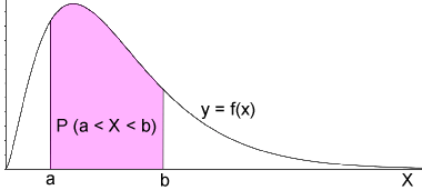
The probability that an outcome, X, lies between the interval a and b is represented by the shaded area under the curve, which can be found by computing the integral of the pdf over the given interval. In other words,

Note that if a were -∞ and b were +∞,

This is because the probability over the entire pdf must be equal to 1, since there is a 100% chance that X would lie in this interval if it is a real number.
There are many different types of continuous probability distributions, including a normal distribution, continuous uniform distribution, and chi-squared distribution.
Normal distribution
The normal distribution, also referred to as the Gaussian distribution, or more informally as a bell curve, is one of the most commonly encountered probability distributions. Its informal name is based on the fact that it is bell shaped, though it is not the only type of distribution that is bell shaped. The figure below shows a normal distribution where μ is the mean, and σ is the standard deviation.
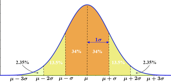
A normal distribution is symmetric about its mean, and most of the values in a normal distribution cluster around the mean, with 99.7% of the values lying within 3 standard deviations of the mean. The further away a value is from the mean, the less likely it is to occur. More specifically, for a continuous random variable that has a normal distribution, 68% of the observations will fall within one standard deviation of the mean, 95% will fall within two standard deviations, and 99.7% will fall within three standard deviations.
The pdf for a continuous random variable that has a normal distribution is

where μ is the mean, and σ is the standard deviation. Like certain other widely used probability distributions, mathematical tables for the values of the cumulative distribution function of the normal distribution exist. The standard normal table, also referred to as the Z table can be used to determine the probability that a value lies within a specified interval in a normal distribution.
One of the reasons that the normal distribution is so important and commonly used is because many physical quantities, such as height and weight, have near normal distributions. Because of this, many statistical tests are designed for use with normally distributed populations. Thus, given that a quantity being studied exhibits a normal distribution, researchers can use many reliable statistical methods to make inferences about the population based on collected samples.
Continuous uniform distribution
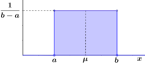
A continuous uniform distribution is a type of symmetric probability distribution that has the following probability density function:

Below is a graphical representation of the pdf of a continuous uniform distribution.
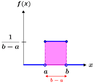
A continuous random distribution is also referred to as a rectangular distribution due to the rectangle formed, as shown by the shaded area in the figure. As the width of the pdf increases, the density of any given value decreases. Also, since all probability density functions integrate to 1 over their respective intervals, the height of the pdf decreases as its width increases. Continuous uniform distributions can be used to describe experiments in which the continuous random variable is symmetric and lies within only a specific interval.
Chi-squared distribution
The chi-squared distribution is one of the most widely used distributions in statistics, particularly for hypothesis testing and the construction of confidence intervals. The pdf for a chi-squared distribution is

where k is the degrees of freedom and  is the gamma function:

It is not always necessary to integrate the pdf of a chi-squared distribution. Like certain other probability distributions, there exist tables that can be used to determine important statistics such as the p-value, which can indicate whether or not a test statistic is statistically significant.